Dimensionality Reduction
When the number of features grows, several things go wrong: data becomes increasingly sparse (the curse of dimensionality), computational complexity grows, overfitting risk increases, distance measures become less meaningful, and visualization becomes impossible. Dimensionality reduction addresses this by projecting data into a lower-dimensional space while preserving as much information as possible.
PCA — Principal Component Analysis
Unsupervised, optimal for dense data with approximately Gaussian features. Finds the directions (principal components) of maximum variance and projects onto the top k of them.
Strengths: interpretable components, mathematically optimal for linear reduction, widely supported.
Limitations: assumes linear relationships; sensitive to outliers; information is lost — you choose how much to sacrifice by choosing k.
PCA finds the direction in feature space that captures the most variance. Drag the angle below to rotate a projection axis. Watch how the spread of projected points changes — and notice what happens near 45°.
Green = original points · Purple = projections onto axis
σ² = 1.899
Why does ~45° capture the most?
The two features are positively correlated — points stretch diagonally. The axis aligned with that diagonal captures the longest spread. PCA finds this automatically.
The math
Var(Xw) = wᵀΣw
- w — the unit vector defining the axis direction
- Σ — the covariance matrix: captures how every pair of features varies together
- wᵀΣw — the variance of the data after projecting onto w
- ‖w‖ = 1 — we constrain the axis to be a unit vector so that length doesn't inflate the variance
Maximizing wᵀΣw subject to ‖w‖ = 1 is a constrained optimization problem. Using Lagrange multipliers, it reduces to solving Σw = λw — the definition of an eigenvector. The largest eigenvalue λ gives the maximum variance, and its eigenvector is PC1.
Four-step walkthrough of PCA: rotate an axis to see how variance changes, observe the eigenvector decomposition, watch a 2D-to-1D projection with its reconstruction error, then use a scree plot to choose k.
t-SNE and UMAP are nonlinear methods designed to preserve local structure — nearby points in high dimensions stay nearby in the projection. Both are excellent for visualizing clusters and structure in high-dimensional data.
Critical distinction: t-SNE and UMAP are visualization tools, not feature extraction tools. Use them to see structure in your data. Don't use them as preprocessing steps for downstream prediction — the axes have no stable interpretation, and results can change with different random seeds. UMAP tends to preserve global structure better than t-SNE and runs faster; it's increasingly the preferred choice for exploration.
Two other methods worth knowing: Truncated SVD works like PCA but on sparse data — use it for TF-IDF vectors. Linear Discriminant Analysis (LDA) is supervised and finds axes that maximize class separation — use when you have class labels and want dimensionality reduction that's class-aware.
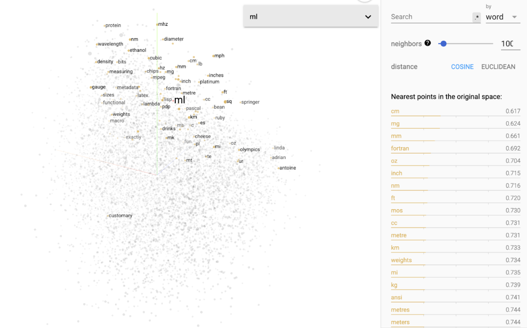
Compare Methods Interactively
The TensorFlow Embedding Projector (projector.tensorflow.org) lets you compare PCA, t-SNE, and UMAP on the same data interactively. Seeing how different methods organize the same high-dimensional space is one of the fastest ways to build intuition about what each method is preserving and what it's discarding.